
By: Denekew A. Jembere
 Licensed under a Creative Commons Attribution-NonCommercial-ShareAlike 4.0 International License.
Introduction
A safer strategy to reduce and prevent crimes plays an important role in increasing the emotional freedom of people to let them focus on their daily productive activities and avoid worries about criminal activities in their surroundings. In addition, reduction and prevention of crimes save law enforcement resources with a stretched positive impact of saving lives which would have been lost during crimes or when fighting criminal activities. In this regard, using historical crime data and applying data mining algorithms help to build models that could predict potentially criminal activity in a given time and location. Therefore, this article outlines an approach to build crime location prediction models; comparing the prediction accuracy of these models; and, proposing the one that comparatively performs well for crime location prediction.
Data Preparation
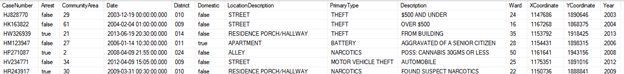
For the data analysis using different data mining algorithms and find some hidden patterns from the huge amount of historical data, this article uses crime data from the city of Chicago (Data.gov, 2018). The original data available in the comma-separated value (CSV) format, got imported into a SQL database table and an initial assessment of the data got performed.
To get the crime data ready for mining, more than 1.8Million records, having misplaced column values, of the 6.7million got fixed pushing subsequent column values and splitting the last column values into the last three columns. Furthermore, due to server performance issues, using the full data for data mining was taking hours to complete training and testing simple clustering. As a result, after additional data preparation and cleaning steps, using the technique suggested by Colley (2014), one percent of the cleansed dataset got randomly selected and a total of 64902 records got inserted into a new table, using the SQL script shown in Figure 1.
| SELECT TOP 1 PERCENT * INTO [CrimesOnePercent] FROM [dbo].[CrimesSince2001] ORDER BY NEWID() |
Figure 1. Random data selection SQL script
The research question from the crime data
In their study, Kumar et al. (2017) explained the importance of including the time dimension of a crime data so that crime prediction models, built using spatial (location) distribution of crimes with the temporal (time) dimensions, can effectively identify crime patterns and related activities. In addition, according to Tayebi et al. (2014), location prediction plays a great role in reducing crimes for criminals who frequently commit opportunistic and serial crimes take advantage of opportunities in places they are most familiar with as part of their activity space. As a result, given input attribute values of a crime data, predicting the location (or x-y coordinates) of the crime will be the focus (the research question) of this article.
For creating different data mining prediction models, to compare and recommend the best performing model, 13 attributes (from the total 20 in the original dataset) that could describe each crime and its location details got selected. The resulting dataset schema looks like Figure 2.
The Data Mining Algorithms and Tools
Among the different data mining algorithms (Guyer & Rabler, 2018) supported by the Microsoft SQL Server Analysis Service (SSAS), three of the algorithms (Clustering, Neural Network, Logistic Regression) were used to create models using the crime dataset.
Clustering Algorithm
The clustering algorithm is used for segmenting or clustering an input dataset into smaller groups or clusters that contain data having similar characteristics. According to Guyer and Rabler (2108), the clustering algorithm, unlike the other data mining algorithms, doesn’t need a predictable attribute to be able to build a clustering model and this approach is used for exploring data, identifying anomalies in the data.
Neural Network Algorithm
According to Guyer and Rabler (2108), the neural network algorithm works by testing each possible state of the input attribute against each possible state of the predictable attribute and calculating probabilities for each combination based on the training data. A model created using this algorithm can include multiple outputs, and the algorithm will create multiple networks.
Logistic regression Algorithm
The logistic regression algorithm has many variations in its implementation and is used for modeling binary outcomes with high flexibility, taking any kind of input and supporting several different analytical tasks. The Microsoft version of this algorithm (the one used here), according to Guyer and Rabler (2108), is implemented by using a variation of the Microsoft Neural Network algorithm.
The Data Mining Tools
To create, train and test the data mining models, using the aforementioned algorithms, the tools used are Microsoft Excel 2013; Microsoft Visual Studio 2017; Microsoft SQL Server Management Studio (SSMS); the Microsoft SQL Server; and, Microsoft SQL Server Analysis Services.
The model building and analysis
To create, train and test the prediction models using the Clustering, Neural Network, Logistic Regression algorithms, the 20 attributes of the sample dataset, CrimesOnePercent, got identified as Key, Input and Predictable, as shown in Table 1. In addition, the total records of the dataset, 64902, got divided into 70% and 30% for model training and model accuracy-test sets, respectively, which gets randomly partitioned by SSAS during the model building.
Table 1.
Key, Input and Predictable attributes of CrimesOnePercent
| Attribute Type | Attributes Detail |
| Key | CaseNumber |
| Input | Arrest, CommunityArea, Date, District, Domestic, LocationDescription, PrimaryType, Description, Ward, Year |
| Predictable | XCoordinate, YCoordinate, |
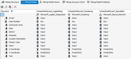
Using the Microsoft Visual Studio 2017, three mining models for the three algorithms got created, as shown in Figure 3, with the Date (Date type), X Coordinate (long type) and Y Coordinate (long type) continuous attributes. To avoid using the default cluster size, which is 10, the Microsoft Excel data mining add-in is used to cluster the data without prediction and get the suggested number of clusters from Excel. As a result, Excel’s cluster count result, which is 13, is used as input in the clustering model building.
Analyzing the resulting models
According to Miliener et al. (2018), a predictive lift score of a model is the geometric mean score of all the points constituting a scatter plot in the predictive lift chart. This score value helps to compare models by calculating the effectiveness of each model across a normalized population. As a result, the deployed models’ detail is analyzed based on their respective lift chart score, which is the average predictive lift of the model measure at each prediction point on the scattered plot. The lift chart score of the models built using clustering, logistic regression, and neural network is 2.09, 2.32 and 4.14, respectively as shown in Figure 4.
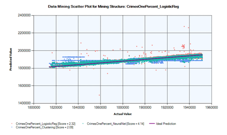
Since it is difficult to see how close to or far from the ideal prediction line, is each model’s prediction point in a single lift chart, Figures 5, 6 and 7 show the respective model’s prediction lift score and scattered points against the ideal prediction line.
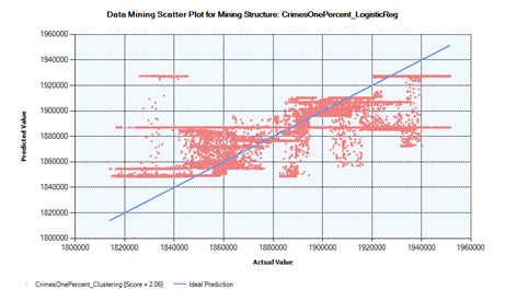
As can be seen in Figure 5, the lower prediction lift-score, 2.06, coupled with most of the points being scattered farther from the ideal prediction line show that the model built using the clustering algorithm can’t predict the crime location x-y coordinates as good as the other models.
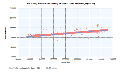
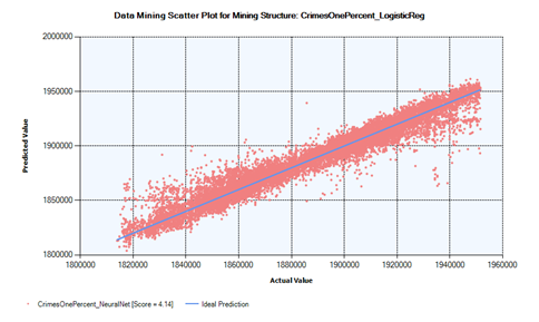
As noted in the brief summary of the algorithms, the logistic regression implementation used here is a variation of the neural network algorithm, the models built using these two algorithms predict well with the predicted points scattered close to the ideal prediction line. More specifically, the model built using the neural network algorithm having the highest lift score, 4.14, predicts a crime location’s x-y coordinate values better than all the three models and hence, this model can further be tuned and tested using the full crime data.
Future Improvement
Since the full historical crime data has location longitude and latitude, the map of Chicago can be created populating locations with the crime location data, which could show the crime clusters visually. Creating such a map would augment the validation of the crime location prediction to help reduce and prevent potential crimes.
References
Colley, D. (2014, January 29). Different ways to get random data for SQL Server data sampling. Retrieved from MSSQLTips: https://www.mssqltips.com/sqlservertip/3157/different-ways-to-get-random-data-for-sql-server-data-sampling/
Data.gov. (2018, August 9). Crimes – 2001 to present. Retrieved from Data Catalog: https://catalog.data.gov/dataset/crimes-2001-to-present-398a4
Guyer, C., Rabeler, C. (2018, April 30). Data Mining Algorithms (Analysis Services – Data Mining). Retrieved from Docs.Microsoft.Com: https://docs.microsoft.com/en-us/sql/analysis-services/data-mining/data-mining-algorithms-analysis-services-data-mining?view=sql-server-2017
Kumar, G., Kumar, N., Sai, R. (2017). Mining regular crime patterns in spatio-temporal databases. International Conference of Electronics, Communication and Aerospace Technology (ICECA), 231.
Miliener, G. Guyer, C., Rabler, C. (2018, May 7). Lift Chart (Analysis Services – Data Mining). Retrieved from Docs.Microsoft.Com: https://docs.microsoft.com/en-us/sql/analysis-services/data-mining/lift-chart-analysis-services-data-mining?view=sql-server-2017 Tayebi, M.A., Ester, M., Glasser, U., Brantingham, P.L. (2014). CRIMETRACER: Activity space based crime location prediction. IEEE/ACM International Conference on Advances in Social Networks Analysis and Mining (ASONAM 2014), 472.